I) Developing a scripted model
Now you know how to record and run Python commands in Abaqus and what commands you can directly adapt from the recordings. You also have learned how to create sets and surfaces, and do evaluations that could not be directly taken from the recorded commands. So you are prepared to use these skills to build a complete Abaqus model that is scripted in Python.
You could just sit down and start developing your code. However, there is a workflow that evolved for me over the years that I will state in the following. Some of it is based on my personal preferences so once you get a hang of it, of course, you can and should adapt it to your needs. But for starting to script Abaqus, I advise you to use the following workflow, particularly so you do not forget about some necessary steps that could cause you troubles later. Also, be aware that you will spend dozens of hours on developing models like that, most of it looking for errors and correcting them: So if you work as structured and clean as possible, this saves you a lot of time (and worries).
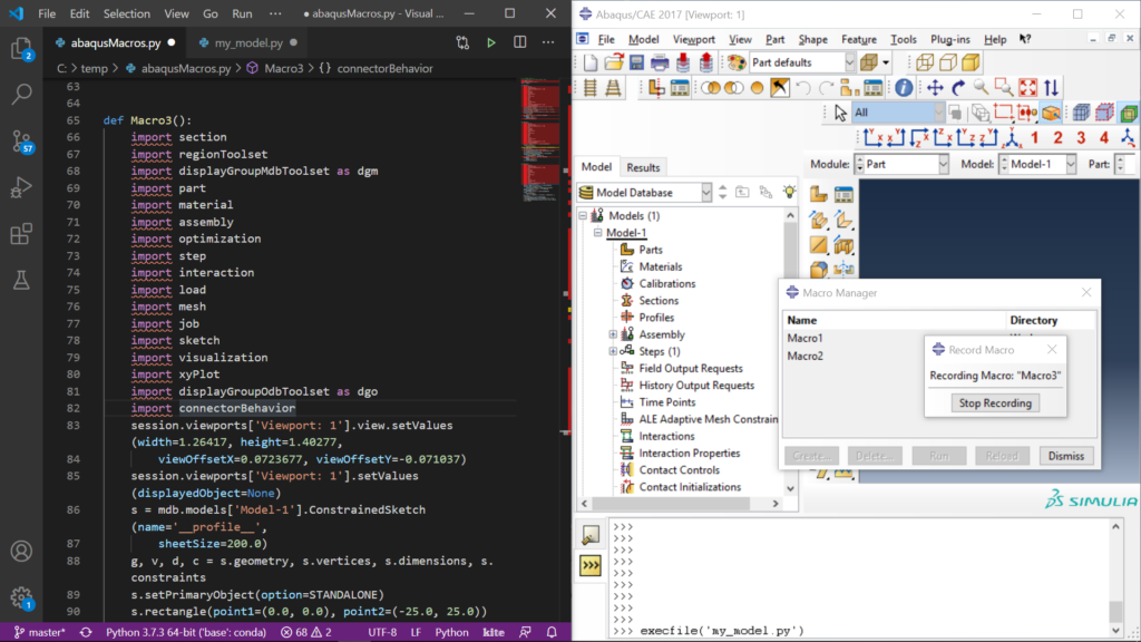
As you record commands and build the scripted model (which we will call model.py), have an Abaqus CAE window open and a text editor (I prefer editors that support syntax highlighting like VisualStudio Code or PyCharm) open side by side. If you use the student version, you can only obtain the Python commands using the Macro manager. Otherwise, you can also look at the jnl file for Abaqus CAE commands and the rpy file for viewer commands. In this setup, we will create the model feature by feature in Abaqus CAE, and stop after each step to copy the new Python code to our model.py, adapt them, test them by running execfile('model.py') in the Abaqus command window (>>>), and continue.
Development environments like Visual Studio Code or PyCharm help you a lot while developing your Python code: They can do code completion, highlight possible errors and so on. They do, however, not know all the Abaqus-Python commands. Tools like kite, however, can learn the Abaqus commands, so once you typed an Abaqus-Python command, it will suggest it in the future when you use code completion.
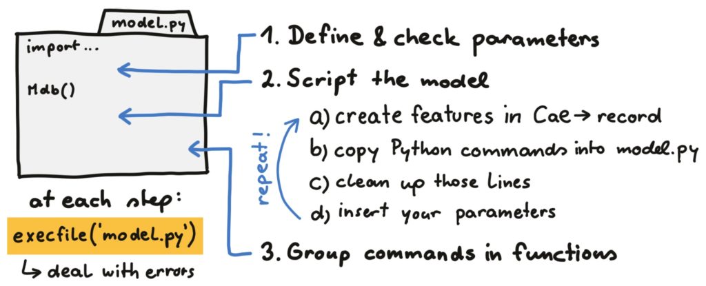
In the following figure, the important steps of the workflow for developing your model.py file are listed. You start from a template that already has all the necessary import statements. As the first step, you define all your model parameters and run some sanity checks on them, so you won’t spend hours looking for an error in your scripted model until you find out that your parameters didn’t make sense. The second step is actually building up your model, which you should do step by step: a) add one or two features in Abaqus CAE, b) copy the recorded lines into your model.py file, c) clean up those lines, and d) insert your model parameters. Then you run your new model.py file in Abaqus CAE either by writing execfile('model.py') in the Abaqus command window (>>>) or by clicking File/Run Script. If everything runs ok, you can continue, otherwise, you have to look for errors in your code, try correcting them, rerun the model and so on.
Once you have completed scripting the model comes the third step: Group all commands in functions to make your code easier to read and more structured. I even suggest having one function in the end that builds, runs, and evaluates your whole model.
Now we look into these steps in more detail, starting from the model header. It contains all necessary import statements (so you can ignore the import statements in the recorded files). We need the TOL variable and the journalOptions command for selecting stuff as stated in chapter 4. Having our working directory defined as DIR0 will help us in the next chapter. Do not forget to describe your model in the first line comment. I also like to add a date, and when I might share it with somebody, my initials MP.
# insert meaningful definition of the model, MP, 09-2020
from abaqus import *
from abaqusConstants import *
from caeModules import *
import os
import numpy as np
session.journalOptions.setValues(replayGeometry=COORDINATE,
		                 recoverGeometry=COORDINATE)
TOL = 1e-6
DIR0 = os.path.abspath('')Code language: Python (python)
1) Define and check parameters
When you got this far, you should already have a sketch of your model with all its parameters defined. At this point, you write them into your model.py file. Do not forget to state the dimension system you are in (e.g. N-mm-s) and add comments for all the variables. This is so you can be sure that when you continue developing your code, you do not have to deal with errors you made here, because you mixed up variables or stated some of them in cm and others in mm.
# parameters for geometry, material, load and mesh (N-mm-s)
# ------------------------------------------------------
b = 10.               # width of the plate (mm)
h = 20.               # height of the plate (mm)
# ...Code language: Python (python)
Because we really don’t want to look for problems later that had to do with parameters that did not make sense, I suggest adding some sanity checks to your model script after the parameter definitions. Particularly for geometric parameters, I suggest doing so! You can choose for yourself how detailed you want to do that: Everybody knows, for example, that the Young’s modulus needs to be positive: So that would be an error you could directly see when you look at your parameters. This is the syntax for checking a variable and raising an error:
if b < 0:
    raise ValueError('width b must be positive')Code language: Python (python)
2) Script the model
Now everything is ready to build the model. Take these lines to reset the model and defining the main model as model.
# create the model
# -------------------------------------------------------
Mdb()                 # reset the model
model = mdb.models['Model-1']Code language: Python (python)
Run the existing Python model in Abaqus CAE with execfile('model.py') in the Python command line. Add one or two features in the Abaqus CAE window. Copy the relevant lines from the rpy, jnl or macro file to your model.py file. Check if this runs. For drawing a rectangle in a sketch, this might look like that:
mdb.models['Model-1'].ConstrainedSketch(name='__profile__',
    sheetSize=200.0)
mdb.models['Model-1'].sketches['__profile__'].rectangle(
    point1=(0.0, 0.0), point2=(35.0, 25.0))Code language: Python (python)
The import statements are 1 big part of the recorded commands. After importing everything from
abaqus,abaqusConstantsandcaeModules, as done in the above header, you do not need those individual import statements.
Introduce shorter variables for the model, sketch, etc. and replace numbers by your variables. Add comments to the code:
# create a sketch
s = model.ConstrainedSketch(name='plate', sheetSize=200.0)
# draw a rectangle
s.rectangle(point1=(0,0), point2=(b,h))Code language: Python (python)
Run the whole script that now contains some new lines. Does it work? Does it do as it should? You will spend most of your time at this step, looking for errors. Abaqus usually tells you where the error occurred. In this case, for example, the sketch was not defined before drawing a rectangle in it:
>>> execfile('model.py')
A new model database has been created.
The model "Model-1" has been created.
File "model_plate.py", line 38, in <module>
    s.rectangle(point1=(0.0, 0.0), point2=(35.0, 25.0))
NameError: name 's' is not definedCode language: Python (python)
If you do not instantly get what is wrong with your code, go back to the last running version and then continue in very small steps (adding and running the script) to find out where exactly the problem was.
Once your newest commands work, continue building your model by recording the next steps of your model creation, job creation and model evaluation.
To create, run, and evaluate a model in one script, Python should wait for the job to complete before doing the evaluation of the odb. This can be done by
job.waitForCompletion()if the job has been defined asjob.
3) Group commands in functions
Once you made sure that parts of the code really work, you can start collecting them in functions. Think of all the variables that you have to pass to the function and what the function should return. In most cases, you will pass the model and some other parameters to the functions that will change the model. You do not need to return the changed model.
def draw_sketch(model,b,h):
    # create a sketch
    s = model.ConstrainedSketch(name='plate', sheetSize=200.0)
    # draw a rectangle
    s.rectangle(point1=(0,0), point2=(b,h))
    returnCode language: Python (python)
Introduce one function that builds, runs and evaluates your whole model by calling all the other functions. If you want, you can keep some order by grouping parameters that belong together in the function arguments (geometry, material, load, etc.):
# function for the whole model
def make_model((b,h),(E,nu),u_y,mesh_size):
    # reset model
    Mdb()
    model = mdb.models['Model-1']
    # call other functions to build the model
    # ...
    returnCode language: Python (python)
This might seem unnecessary to you, and introducing lots of arguments of functions where we input variables that we defined in a fixed way above seems useless. But keep in mind what we want to do ultimately: Varying some of our parameters in an automated way, and this is much easier once we have to call one function of the model and not make a loop over more than hundred lines of code.
II) Scripting the example model
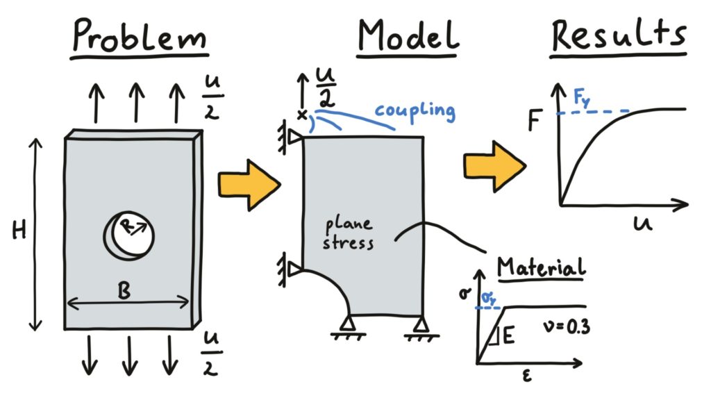
The figure below shows the model we introduced in chapter 2. All the parameters except the plate thickness T are stated in the figure. The boundary conditions look good (no rigid body motion expected) so we can start scripting the model. We start by creating an Abaqus Model by clicking in Abaqus CAE. This is the time to look if the model runs, not during scripting. Once everything is working (as in this cae file), you can start building your scripted model.
a) Header and variables
We take the header of the script from above and insert a meaningful name, my initials and a date:
# Plate with hole model for Abaqus/Python course, MP, 10-2020

from abaqus import *
from abaqusConstants import *
from caeModules import *
import os
import numpy as np
session.journalOptions.setValues(replayGeometry=COORDINATE,
		                 recoverGeometry=COORDINATE)
DIR0 = os.path.abspath('')
TOL = 1e-6Code language: Python (python)
We state that the parameters are given in the N-mm-s system and define all of them. Taking time to write comments for all those parameters and writing down their dimensions helps you avoid errors. In this case, we check if the hole is really inside the plate: If not, we return an error.
# parameters for geometry, material, load and mesh (N-mm-s)
# ------------------------------------------------------
b = 16.               # width of the plate (mm)
h = 20.               # height of the plate (mm)
radius = 4.5          # radius of the hole (mm)
uy = 0.08             # vertical displacement of the top (mm)
E_steel = 210000.     # Young's modulus of steel (MPa)
nu_steel = 0.3        # Poisson's ratio of steel (1)
sy_steel = 500.       # yield stress of steel (MPa)
mesh_size = 0.3       # edge length of the mesh (mm)

if radius >= b/2:
    raise ValueError('width b too small for the hole radius')
if radius >= h/2:
    raise ValueError('height h too small for the hole radius')Code language: Python (python)
Already structuring the code by grouping commands and writing headers makes it easier to find problems in your code and later helps you for creating functions.
b) Model setup
We next take the template for resetting and redefining the model as model and add it to the model.py script:
# create the model
# -------------------------------------------------------
Mdb()                 # reset the model

model = mdb.models['Model-1']Code language: Python (python)
Now its time for recording commands in Abaqus CAE and copying them into the model.py file. I created a sketch and drew the geometry of the plate in it, which consisted of four lines and one arc. After cleaning up the code and removing lots of unnecessary constraint commands, the sketch can be built like this:
# draw the sketch
s = model.ConstrainedSketch(name='plate', sheetSize=200.0)
s.ArcByCenterEnds(center=(0,0), point1=(0,radius), point2=(radius,0),
                  direction=CLOCKWISE)
s.Line(point1=(radius,0), point2=(b/2.,0))
s.Line(point1=(b/2.,0), point2=(b/2.,h/2.))
s.Line(point1=(b/2.,h/2.), point2=(0,h/2.))
s.Line(point1=(0,radius), point2=(0,h/2.))Code language: Python (python)
As described above, this yielded from iteratively changing and running the code and checking what it did in Abaqus CAE. Creating the part is fairly simple, and was adapted to those lines:
# create the part
p = model.Part(name='plate', dimensionality=TWO_D_PLANAR,
               type=DEFORMABLE_BODY)
p.BaseShell(sketch=s)Code language: Python (python)
As we discussed in chapter 3, the trickiest part of scripting the model is creating sets and surfaces. I did not record any commands for that but used the commands that were introduced in chapter 3 for selecting all faces, edges by their bounding box, and a reference point in this weird (but necessary) syntax:
# create sets, surfaces, and reference point
p.Set(name='all', faces=p.faces[:])
p.Set(name='x_sym', edges=p.edges.getByBoundingBox(xMax=TOL))
p.Set(name='y_sym', edges=p.edges.getByBoundingBox(yMax=TOL))
p.Set(name='top', edges=p.edges.getByBoundingBox(yMin=h/2.-TOL))

rp = p.ReferencePoint(point=(0,h/2,0))
p.Set(name='RP', referencePoints=(p.referencePoints[rp.id],))Code language: Python (python)
The commands for creating materials, creating sections and assigning sections is straight-forward again. Just record the commands and clean them up.
In the recorded commands, you will have lots of additional options like the
thicknessinHomogeneousSolidSection: You can just keep all of them, which makes your code bulky and confusing — Or you try removing some that seem irrelevant and check if your script still works.
# create material, create and assign sketchOptions
mat = model.Material(name='steel')
mat.Elastic(table=((E_steel, nu_steel), ))
mat.Plastic(table=((sy_steel, 0.0), ))

model.HomogeneousSolidSection(name='steel', material='steel',
                              thickness=None)

p.SectionAssignment(region=p.sets['all'], sectionName='steel',
                    thicknessAssignment=FROM_SECTION)Code language: Python (python)
The next step is defining the assembly as a and creating an instance of your part:
# assembly
a = model.rootAssembly
inst = a.Instance(name='plate-1', part=p, dependent=ON)Code language: Python (python)
Then we record and adapt the commands for creating a static load step and create a history output for the reference point. For the history output, as for boundary conditions and loads, we have to use the instance and not the part (inst.sets['RP']):
# step and history output
model.StaticStep(name='pull', previous='Initial', maxNumInc=1000,
                 initialInc=0.1, minInc=1e-08, maxInc=0.1, nlgeom=ON)

model.HistoryOutputRequest(name='H-Output-2', createStepName='pull',
                           variables=('U2', 'RF2'), region=inst.sets['RP'])
Code language: Python (python)
In the interaction module of Abaqus CAE, we defined a coupling of the upper nodes and the reference point, which corresponds to this recorded command (state with u1=OFF that the 1st Degree Of Freedom (DOF) should not be coupled and with u2=ON that the second DOF should be coupled: in a 3-d model, do not forget the other DOFs):
# constraint
model.Coupling(name='couple_top', controlPoint=inst.sets['RP'],
               surface=inst.sets['top'], influenceRadius=WHOLE_SURFACE,
               couplingType=KINEMATIC, u1=OFF, u2=ON, ur3=OFF)
Code language: Python (python)
We need three boundary conditions in the model: Two symmetries and one vertical displacement at the top. You can record creating one of these boundary conditions, and adapt it for the three of them. Just adapt the createStepName, the region and what displacements are constrained:
# boundaries and load
model.DisplacementBC(name='x_sym', createStepName='Initial',
                     region=inst.sets['x_sym'], u1=0)
model.DisplacementBC(name='y_sym', createStepName='Initial',
                     region=inst.sets['y_sym'], u2=0)
model.DisplacementBC(name='pull', createStepName='pull',
                     region=inst.sets['RP'], u1=0, u2=uy, ur3=0)Code language: Python (python)
For creating boundary conditions in Abaqus CAE, you can use the option Symmetry/Antisymmetry/Encastre: This yields separate commands for each type of boundary condition. I suggest to always use Displacement/Rotation and then set relevant displacements to zero. This always uses the same command
model.DisplacementBC()and is thus easier for scripting the model.
Creating a mesh can get quite complicated. In this case, however, we only want to seed the whole part with an edge length of size and generate the mesh of the plate. For using edge-based seeds or changing the element types (plane stress is the default for 2D elements), you can record and insert additional commands:
# meshing
p.seedPart(size=mesh_size)
p.generateMesh()Code language: Python (python)
So the model is completed! For running it, we create and run a job. If we want to evaluate the results in the same model, we can use the waitForCompletion function so the script waits until the job finishes before it continues:
job_name = 'pull-plate'

# create and run job
job = mdb.Job(name=job_name, model='Model-1', type=ANALYSIS,
              resultsFormat=ODB)
job.submit(consistencyChecking=OFF)
job.waitForCompletion()Code language: Python (python)
Before submitting the job, you can save the model using
mdb.saveAs('model-name.cae'). If the job crashes, you then have the latest cae file to check for errors.
c) Model evaluation
Evaluating the model using Python commands is usually quite different from what you get when you click in the Abaqus Viewer and record commands. Scripting those evaluations is described in chapter 4. We now apply those scripts to the plate model, starting with a small header that loads our odb file, defines the viewport as vp and displays the odb file:
# open the odb
odb = session.openOdb(job_name+'.odb')

vp = session.viewports['Viewport: 1']
vp.setValues(displayedObject=odb)Code language: Python (python)
1) Print field output to an image
In the plate model, we do not want to output the full stress, strain and displacement fields. Otherwise, we would have needed to define additional field output of the coordinates like described in chapter 4. We want, however, create images of the stress fields. For that, we add the commands for setting the size of the viewport to the model script, run it and then rotate, zoom, and drag until we like the view of the model.
# print a field output image
# ------------------------------------------------------

# Change size of viewport (e.g. 300x200 pixel)
vp.restore()
# position of the viewport
vp.setValues(origin=(50,-50))
vp.setValues(width=150, height=200)Code language: Python (python)
Then, we save the view using View/Save with the option Save current. The recording of this command is then added to our script. We only need to use the command vp.view.setValues to load this saved view and we are good to go. If we intend to change the geometry of our model a lot, this fixed view might be ok for some of the options but not for the others. Then, you can set the view to one of the default views (in the code below, it is the Front view) or use the option Auto-fit when saving the view.
# set up in Abaqus Viewer and copied here
session.View(name='User-1', nearPlane=24.242, farPlane=39.003, width=7.2278,
    height=9.3665, projection=PERSPECTIVE, cameraPosition=(2.5, 5, 31.623),
    cameraUpVector=(0, 1, 0), cameraTarget=(2.5, 5, 0),
    viewOffsetX=-1.3504, viewOffsetY=0.25069, autoFit=OFF)

# load the defined view
vp.view.setValues(session.views['User-1'])

# for a varied plate size, take an automatic front view
# vp.view.setValues(session.views['Front'])Code language: Python (python)
Then, we need to define what kind of field output we want to display and for what frame we want to display the results. Those commands can be recorded and copied into the model script.
# view the right field output
vp.odbDisplay.display.setValues(plotState=(CONTOURS_ON_DEF, ))
vp.odbDisplay.setPrimaryVariable(variableLabel='S',
     outputPosition=INTEGRATION_POINT,
     refinement=(INVARIANT, 'Mises'),)
# set the displayed frame
vp.odbDisplay.setFrame(step=0,frame=-1)Code language: Python (python)
There are some view options regarding state blocks and the legend that I like to set. If you would like to keep some of the elements or prefer a different font in the legend, record similar commands as described in chapter 4:
# change the legend and what is displayed
vp.viewportAnnotationOptions.setValues(legendFont=
       '-*-verdana-medium-r-normal-*-*-140-*-*-p-*-*-*')
vp.viewportAnnotationOptions.setValues(triad=OFF, state=OFF,
    legendBackgroundStyle=MATCH,annotations=OFF,compass=OFF,
    title=OFF)Code language: Python (python)
Finally, we can print the view of the field output to a png file. With the imageSize argument, you can change the resolution of the picture. Here, we create a png image that uses the model name with the ending _mises:
# print viewport to png file
session.printOptions.setValues(reduceColors=False, vpDecorations=OFF)
session.pngOptions.setValues(imageSize=(1500, 2000))
session.printToFile(fileName=job_name+'_mises', format=PNG,
		    canvasObjects=(vp,))Code language: Python (python)
2) Evaluating history output
Following the description in chapter 4 on evaluation history output, we here obtain the history region by its name (for other history outputs, look how they are colled in Abaqus by printing step.historyOutputs.keys()):
# evaluate the history output
# ------------------------------------------------------
step = odb.steps['pull']

# query the label of the reference point
inst = odb.rootAssembly.instances['PLATE-1']
n_hr = inst.nodeSets['RP'].nodes[0].label

# put together a string to select history region
str_hr_node = 'Node '+inst.name+'.'+str(n_hr)

# select the history region with the reference point
hr_rp = step.historyRegions[str_hr_node]Code language: Python (python)
The history region then contains the history output, that we access here. We get the data for the vertical displacement (U2) and the vertical reaction force (RF2). Using the syntax of NumPy arrays, we obtain the second column of both displacement and reaction force with the index [:,1] and stack those two columns into a new array res_u_f, that we save in a dat file:
# get vertical displacement and reaction force data
# ((t,u),...), ((t,rf),...)
res_u = np.array(hr_rp.historyOutputs['U2'].data)
res_rf = np.array(hr_rp.historyOutputs['RF2'].data)

# only take the second column of data and stack those columns
res_u_f = np.column_stack((res_u[:,1],res_rf[:,1]))

# write u-rf data to file
np.savetxt(job_name+'_res_u_f.dat',res_u_f)Code language: Python (python)
3) Evaluating field output along a path
Furthermore, we are interested in the stress distribution in the remaining cross-section of the plate. As described in chapter 4, we create a coordinate-based path:
# evaluate the stresses along path (y=0)
# ------------------------------------------------------

# create path from coordinates
pth = session.Path(name='Path-1', type=POINT_LIST,
                   expression=((radius,0,0), (b/2.,0,0)))Code language: Python (python)
To evaluate field output along a path, we must first display the desired field output and set the frame for which we want to get the results:
# field output to be evaluated along path
vp.odbDisplay.setPrimaryVariable(variableLabel='S',
    outputPosition=INTEGRATION_POINT,refinement=(COMPONENT, 'S22'))

# setting the frame for path evaluation
vp.odbDisplay.setFrame(step=0,frame=-1)Code language: Python (python)
And we evaluate the vertical stresses along 20 equidistant points over this path. This means that Abaqus interpolates the stress fields. Stating shape=UNDEFORMED and labelType=X_COORDINATE returns a list of undeformed x-coordinates / vertical stress pairs that we save to a dat file:
# output for 20 equidistant points over path
# shape: path over DEFORMED or UNDEFORMED geometry

n_points = 20

# get vertical stress S22 over X_COORDINATE
xy = session.XYDataFromPath(name='XYData-1', path=pth,
    includeIntersections=False, shape=UNDEFORMED,
    projectOntoMesh=False, pathStyle=UNIFORM_SPACING,
    numIntervals=n_points, projectionTolerance=0,
    labelType=X_COORDINATE)

# write results to file
np.savetxt(job_name+'_res_s22_path.dat',xy.data)Code language: Python (python)
d) Organizing the model using functions
Once you have your model fully scripted and tested some parameter options, it is time to tidy the script up! Collect all the commands that belong together in a function to get a function for geometry, sections, the assembly, boundaries, running the model and your evaluations. Think about what is needed as an argument in each function: The geometry function, for example, would need the model and the geometry parameters as arguments. When a function creates something (like a part) that is needed in later functions, return this variable.
Create one function for the whole model creation, run, and evaluation that calls all the other functions. Check the model parameters in this function (or write a separate function for checking model parameters and call that function). This function could look like that:
# one function for the whole plate model (create, run, evaluate)
def plate_model(job_name,(b,h,radius),(E,nu,sy),uy,mesh_size):
    # check parameters for errors
    if radius >= b/2:
        raise ValueError('width b too small for hole radius')
    if radius >= h/2:
        raise ValueError('height h too small for hole radius')
    # reset model
    Mdb()
    model = mdb.models['Model-1']
    # make the parts, mesh it and return it
    p = make_geometry(model,(b,h,radius),mesh_size)
    # make materials and sections
    make_sections(model,(E,nu,sy))
    # make the assembly & constraint
    inst = make_assembly(model,p)
    # create step and boundaries
    make_boundaries(model,inst,uy)
    # save the model
    mdb.saveAs(job_name)
    # run the model
    run_model(model,job_name)
    # evaluate: create image
    evaluate_image(job_name)
    # evaluate: history output and path
    evaluate_ho_path(job_name)
    return modelCode language: Python (python)
Note that by writing inst = make_assembly(model,p) you take the returned argument from the function and pass it to the variable inst to be used later. The individual functions are not listed here but can be found in the Appendix.
You might ask yourself why we do not define the set and step names as variables: For a simple script like that, this would only complicate things. Just make sure that you have all your sets and surfaces defined in the geometry function that you will need in the other functions.
You can call the model function just by stating values or variables for the parameters:
# call the model function
plate_model('small-plate',(20.,15.,7.),(1200.,0.3,40),0.05,1.)Code language: Python (python)
If you want to do that for 3 different parameter combinations, just write multiple function calls. If you want to vary a parameter in a certain range and look at model results, you can write a for loop that does that (note that in some way you should remember what job name corresponds to what parameters: Here, we just write the height h into the job name):
# define a list for the height
h_list = [10., 15., 20., 25.]

# a for loop to vary the height in the model
for h in h_list:
    # writing the h value into the job name
    job_name = 'plate-h-'+str(int(h))
    plate_model(job_name,(20.,h,7.),(1200.,0.3,40),0.05,1.)Code language: Python (python)
Now, this is what we all have been waiting for! You have all the parameters at your fingertips and can vary whatever you want. The sky computation time is the limit! You can find the full script of the model using functions here.
Exercises
Now the time has come to script your own model. As you have practised in the last two chapters on small model details, you will now do for your whole model.
- Collect all parameters of your model and write the part of your model script where you define all those parameters and do some sanity checks.
- Build up your scripted model feature by feature as described above. Test this after each step.
- Build up your evaluation as described above and with help from the previous chapter. Test some different kinds of parameter sets and look at the results. Did you expect that?