Have you ever seen someone presenting a finite element model where you didn’t have any idea what they actually did and what the aim of the whole work was? And wondered what all those fancy diagrams and colorful pictures were for?
This chapter is about developing a finite element model from an engineering problem in a neat and structured way, so you won’t do presentations like that. You will learn to be aware of the aim of the analysis at all times and see the big picture, of which the FE model is only a small part.
Maybe you work in a project where computing stress fields in a certain component is your task. Which is definitely not the big picture: What are the stresses for? Is there a critical deformation, and do we care about the component breaking? What do the stresses mean, and what could be changed in the component? Are we interested in material alternatives, etc.? You can still think about those questions, and if your supervisors did not already tell you (or even know) what the model is for, you can tell them!
I) Modelling Scheme
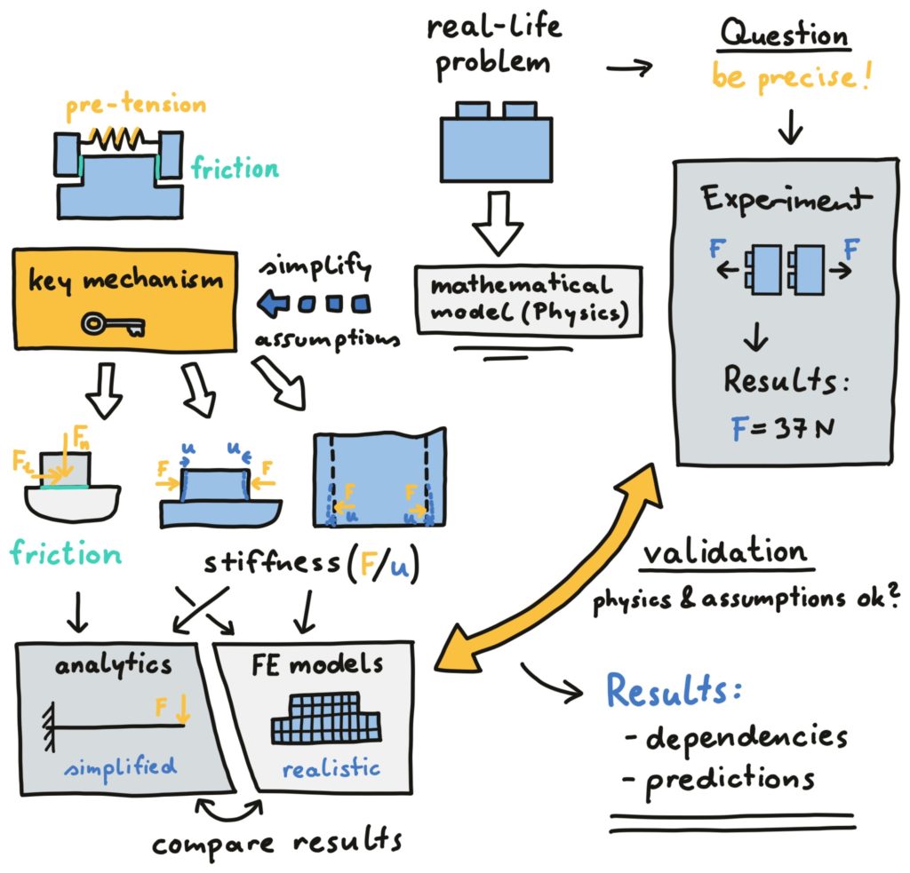
Here you see a scheme of how we start from a real-life problem and develop analytical and FE models for them. As you can see, there is much work to be done before we get to building the FE model: We have to think of a precise question to ask; think of a way test it; simplify the problem to get a key mechanism; and develop analytical and FE models to capture this key mechanism. In the end, we validate our model by comparing model results and test results.
a) Identify Problem, Mathematical Model
Now let’s look at a scheme for building a model starting from a real-life application in the figure above. In the beginning, we need to ask a specific question about that application which can lead us to the engineering problem. “What is the stress field?” is NOT a valid question! Be more specific and ask about something on the application scale (deformation, failure, etc.) like “Does the component fail under those loads?”. Next, we have to think about a mathematical model for answering that question. What kind of physics have to be in the mathematical model: Mechanics, heat transfer, fluid mechanics, electromagnetics?
b) Test it: The Experiment
Think of how you could make a test to answer that question. In this course, we do that using stuff you have at home (string, weights, a scale, duct tape, etc.)! You do not have a 700 kg railway wheel at home? Think of something similar! A fascial roll or cooked noodles make a good cylinder with strains you can actually see! Those tests are not professional? They’re not, but you will understand your problem! What did you expect to happen in the test and what do you observe?
c) Simplify: Key Mechanism
Once we are sure about our physics and have seen first test results, we need to break down the problem as much as possible: No matter how complicated it looks, reduce it to the key mechanism! There is a temperature-dependence of the material stiffness and tolerances in the geometry? We don’t care! Is there a 1-dimensional model that does something similar? Sounds good! You can explain the core mechanism in two sentences to your grandmother? Sounds even better! Don’t worry if this seems hard: It’s the hardest but also the most important step in your analysis. Just try some things out and see if you can still take something away. Once you can’t you are there! Make a list of your simplifications and assumptions to possibly add later. All these assumptions will be checked when we validate our model using model results and test results.
d) Divide Mechanisms
When you have reached your key mechanism, it’s time to divide it into different aspects and maybe add some of the features we removed before. Think already about different kinds of analytical models to calculate stiffness or stress values. Define how they would fit together. What kinds of simplifications do you have to make to calculate it analytically? Do you over- or underestimate your stresses and deformations with those simplified models? Are your models the “worst-case scenario”? For what aspects will we need the FE method for accurate results?
e) Analytical Models
Now set up and solve your analytical models. Even though they oversimplify your problem, you will get some dependencies and starting points for your FE models. Think about what your results tell: What exponents do your parameters have in the formulas? Which are the most important? Were there some dependencies in the experiments you can qualitatively explain in that way?
f) Finite Element (FE) Models
At that point we can start setting up the FE models: Did you notice how long it took us to get here? But did you notice how much we already know about our problem? From the analytical models, we already know well what results to expect. And we only use FE models for issues where either geometry, material, boundary conditions, or loads are too complicated for making quantitative predictions in analytical models.
Even here, you should start with a pencil before you build your model in the FE software. Draw your model with all boundary conditions, constraints, loads, contact definitions, and define your material model. Think about what dimensionality to use (3D, axial-symmetric, plane stress, or plane strain) and what kind of elements (solid, shell, beam) you want to use. Is your drawing complete and are the assumptions reasonable? Are there errors in your boundaries and loads (like rigid body motion)?
Once you have a complete and valid sketch of your FE model, set it up in the software of your choice. Make the usual checks concerning deformation fields (are the boundary conditions you wanted to apply actually applied?) and mesh size. Run the model and obtain the model results.
g) Errors in FE Model?
Once your FE results come in, see if they fit with the analytical results. Can the differences be explained by the assumptions of the analytical model? Does the deformation field of the FE model make sense? This is to check if you have set up your model right. My rule of thumb is: For every feature that is new to me, I need at least four tries until I get it right.
h) Validation
Finally, you have FE results that look ok and analytical results predicting dependencies. What we do not know yet is if our mathematical model was right and if our key mechanism is relevant for what happened in the tests. To check that, we compare model results to test results to validate the model. Are there dependencies of your model that were not investigated in the tests? Think of additional tests to study them! When the results fit reasonably well, our model is validated: That means that analytical dependencies apply and the model can predict what is happening in the tests. If the model results do not fit well with the test results, you need to get back to your key mechanism and rethink your assumptions and simplifications: Was there something you disregarded but might be relevant? Something that might explain the differences in model and test? Start a second loop with an adapted key mechanism and see if this one fits better with the observations of the test.
II) The example problem
For automizing our Abaqus models, I thought of a small real-life problem. There were strips of sour candy (by Haribo, Cola flavour) lying around, and I asked myself what would happen when they have a hole in them and are pulled. We are interested in where they break and what forces and elongations we reach. As you can see in this video, they deform quite a lot until they break next to the hole:
Following the explanation above on modelling, we can think of an experiment and about the key mechanism. We are in the world of mechanics, and the principal mechanism is a stress concentration that becomes less and less pronounced due to ideal plastic behaviour. Also, there is a plastic necking of the two sides of the hole, which ultimately leads to failure.
a) The experiment
In the experiment, I wanted to measure both the elongation and the force. Not having a tensile test machine at home, I found a scale in my kitchen and some graph paper. When I stick the stripe under something heavy on the scale and pull it upwards, the reduction of the weight on the scale corresponds to my force. Having a graph paper in the background, I can see the elongation in a video that I made. The testing jig looked like that:
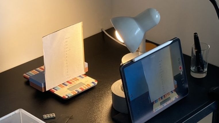
I manufactured four specimens, clamped the upper end between two Lego bricks, and then pulled on the candy stripe. This is a video of specimen number 1:
For specimen 2, I was too fast for the scale to display the weight and for specimen 4, the stripe failed in the clamping. That means that only specimens 1 and 3 are valid. Those are the force-elongation curves I got for specimen 1,3 and 4 by stopping the video and writing down displacement and force values:
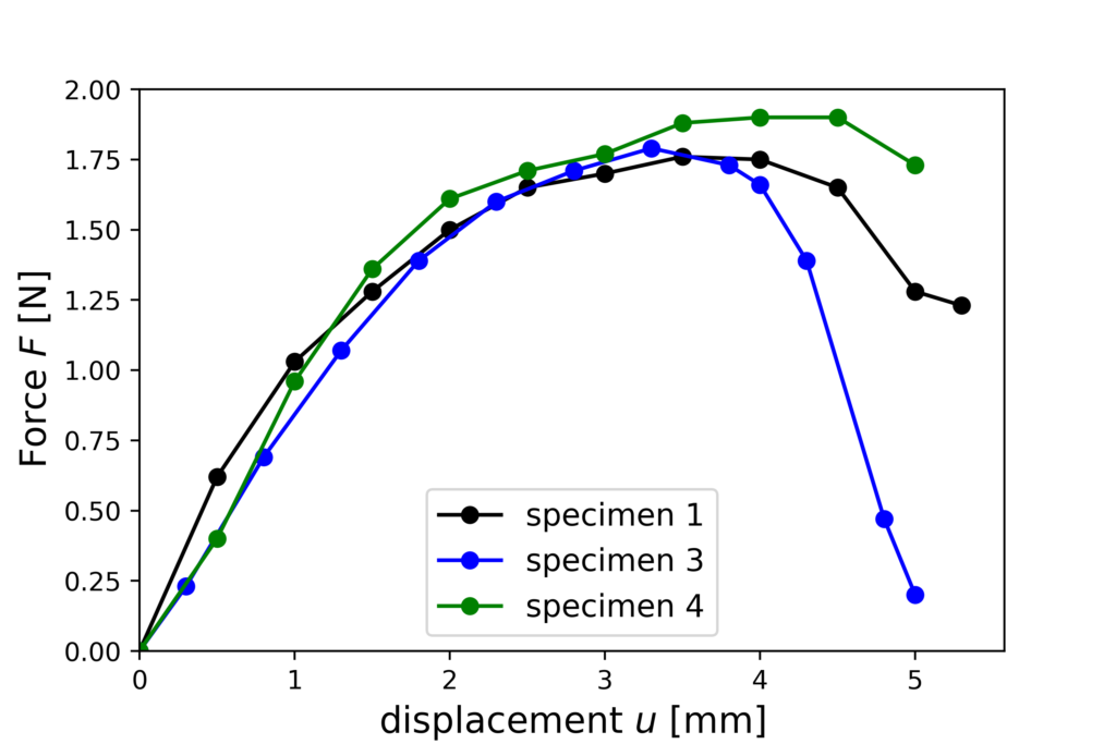
The curves are surprisingly reproducible! We see a more or less linear increase in the force up to an elongation (displacement) of about 1.5 mm, and then some kind of plateau with a subsequent drop in the force.
b) Analytical models
For the onset of plastic deformation, we have the formulas for stress concentrations that we can use. For the plastic collapse (maximum force) we can just assume that the whole cross-section has reached the yield stress. Those two calculations are assuming small deformations. The actual cross-section, however, would be considerably lower and those formulas will overestimate the forces. To consider big deformations, we will use the FE model and not try to adapt our analytical models.
For small holes, the maximum stress due to the stress concentration is:
\cfrac{\sigma_{max}}{\bar{\sigma}}=1+2\sqrt{\cfrac{c}{r}}
with the mean stress next to the notch \bar{\sigma} and the notch width c and notch tip radius r. In our case of a round hole, c=r so that the maximum stress is three times the mean stress.
The mean stress can be calculated as the force divided by the cross-section area A=T*(B– 2R), with T denoting the specimen thickness. So the force for the onset of plastic deformation (first force when the yield stress is reached) F_{yield} becomes
F_{yield}=\cfrac{\sigma_y}{3}\; T \left(B-2 R\right)
For the plastic collaps, the force is by a factor of 3 higher:
F_{collapse}=\sigma_y\; T \left(B-2 R\right)
That means that if we have only small deformations but ideal plastic material behaviour, we predict a first yielding of the specimen at a force that is three times smaller than the force for plastic collapse. This is definitely not the case for out tests and something to further study in the finite element models.
c) Finite Element Model
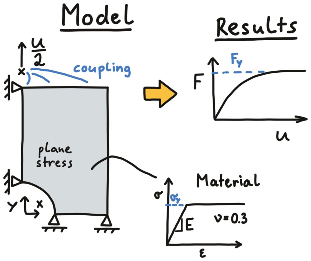
We will only develop a sketch of our model and then continue with building, running, and evaluating the model later. As mentioned above, we want to uniquely define the model setup in one drawing, defining geometry, constraints, boundary conditions, loads, and also the material model.
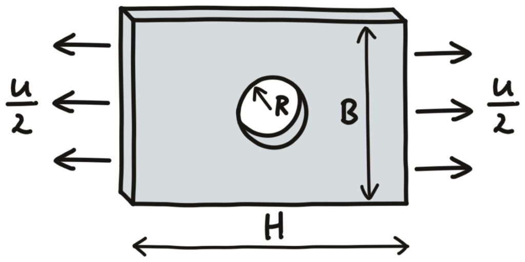
The model is defined with the plate height H, width B, and thickness T, the radius of the hole R, and displacement u from above. The Young‘s modulus E, Poisson’s ratio \nu, yield stress \sigma_y are stated in the following image. We are interested in the plastic strains and the force/displacement curve of the plate. The two symmetry boundary conditions hinder any rigid body motion. The coupling of the top nodes is done for the y-displacements.
Exercises
- Think about one application from your hobbies where it would be convenient to set up a model and fully automate it. Draw a picture as I did for the example model. Carry out the steps above to do some experiments, find the key mechanism, and do analytical calculations for your model.
- How can the problem be simplified to have less than 1000 nodes in the model? What results are you interested in and what do you think they could be?
- We do not want to think about how to automate the model and how the model should look like at the same time! So check that you have all the important information in your model definition: are all parameters there? Is the dimensionality defined? Are all boundary conditions, interactions, and loads defined? Is the material model fully defined?
- Build your model in Abaqus CAE with typical parameter values. Run the model and look at the results that you were interested in. Remember what you had to do in Abaqus CAE or write it down.